Predicting US Equities Trends Using Random Forests

Jul 1, 2016

Introduction

One of the main reasons I started studying machine learning is to apply it stock market and this is my first post to do so. Specifically, we are going to predict some U.S. stocks using machine leaning models.

Depending on whether we are trying to predict the price trend or the exact price, stock market prediction can be a classification problem or a regression one. But we are only going to deal with predicting the price trend as a starting point in this post. The machine learning model we are going to use is random forests. One of the main advantages of the random forests model is that we do not need any data scaling or normalization before training it. Also the model does not strictly need parameter tuning such as in the case of support vector machine (SVM) and neural networks (NN) models. However, research indicates that SVM and NN achieved astonishing results in predicting stock price movements (1). But we will leave them for another separate post. Manojlovic and Staduhar (2) provides a great implementation of random forests for stock price prediction. This post is a semi-replication of their paper with few differences. They used the model to predict the stock direction of Zagreb stock exchange 5 and 10 days ahead achieving accuracies ranging from 0.76 to 0.816. We are going to use the same methods as the ones in the paper with similar technical indicators (only two different ones) to predict the US stock market movement instead of Zagreb stock exchange and varying the days ahead from 1 to 20 days head instead of just 5 and 10 days ahead.

Research Data

I chose 8 of the top companies in the S&P 500 in terms of market cap: AAP, BRK-B, GE, JNJ, MSFT, T, VZ, XOM.

The data sets for all the stocks are from May 5th, 1998 to May 4th, 2015 with total of 4277 days (the figure above shows a higher range). Since we have 8 stocks and we are going to predict the price movement from 1 to 20 days ahead, we will have a total of 160 data sets to train and evaluate. But before proceeding with training the data, we had to check weather the data are balanced. The figure below shows the percentage of positive returns instances for each day and for each stock. Fortunately, the data does not need to be balanced since they are almost evenly split for all the stocks.

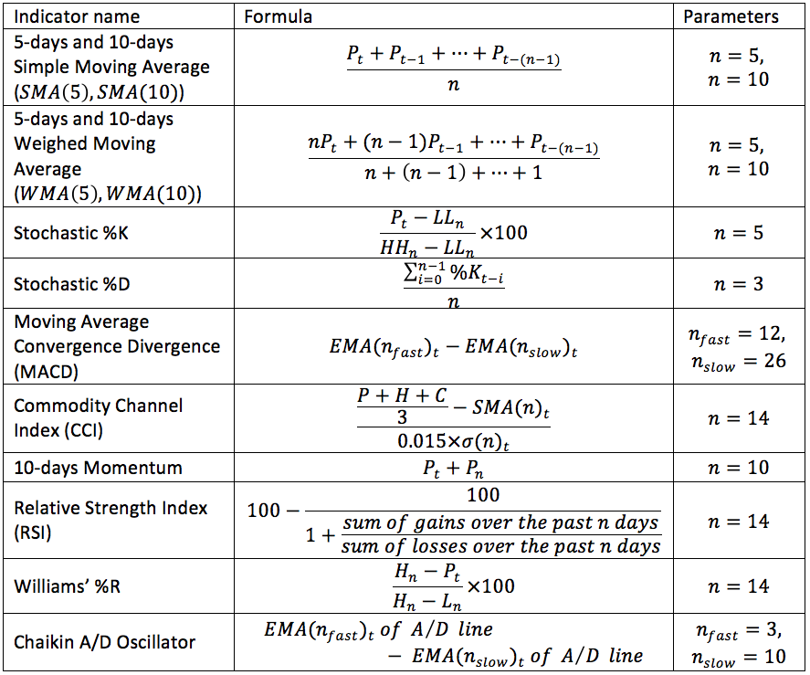
The technical indicators were calculated with their default parameters settings using the awesome TA-Lib python package. They are summarized in the table below where ${ P }_{ t }$ is the closing price at the day t, ${ H }_{ t }$ is the high price at day t, ${ L}_{ t }$ is the low price at day t, ${ HH}_{ n }$ is the highest high during the last n days, ${ LL}_{ t }$ is the lowest low during the last n days, and $EMA(n)$ is the exponential moving average.

Model and Method

As mentioned above, one of the advantages of random forests is that it does not strictly need parameter tuning. Random forests, first introduced by breidman (3), is an aggregation of another weaker machine learning model, decision trees. First, a bootstrapped sample is taken from the training set. Then, a random number of features are chosen to form a decision tree. Finally, each tree is trained and grown to the fullest extend possible without pruning. Those three steps are repeated n times form random decision trees. Each tree gives a classification and the classification that has the most votes is chosen. For the number of trees in the random forests, I chose 300 trees. I could go for a higher number but according to research, a larger number of trees does not always give better performance and only increases the computational cost (4). Since we will not be tuning the model’s parameters, we are only going to split the data to train and test set (no validation set). For the scores, I used the accuracy score and the f1 score. The accuracy score is simply the percentage (or fraction) of the instances correctly classified. The f1 score calculated by

$$F1 =2\frac { precision\times recall }{ precision+recall } $$ $$precision=\frac { tp }{ tp+fp } $$ $$recall=\frac { tp }{ tp+fn } $$

where $tp$ is the number of positive instances classifier as positive, $fp$ is the number of negative instances classified as positive and $fn$ is the number of positive instances classified as negative. Because of the randomness of the model, each train set is trained 5 times and the average of the scores on the test set is the final score. All of the calculation were done by python’s scikit-learn library.

Results

As seen from the two figures above, we get poor results for small number of days ahead (from 1 to 4) and greater results as the number of days ahead increases afterworlds. For almost all the stocks for both scores, the highest scores are in the range of 17 to 20-days ahead.

Conclusion

In this post, we demonstrated the use of one machine learning model, random forests, to predict the price movement (positive or negative) of some of the major US equities. We got satisfying results with ten technical indicators when predicting the price movement mostly within 14 to 20 days ahead witch scores ranging from 0.78 to 0.84 for the accuracy scores and from 0.76 to 0.87 for the f1 scores. We probably could have better results if we add more features that includes fundamentals and macro economic variables. Also, since commodities are highly leveraged, we could use minute by minute data to predict the movement of commodity prices at the end of the day. Actually this was my initial choice of data. But I could not find a source that provides minute by minute data for free.

References

1. Yakup Kara, Melek Acar Boyacioglu, Ömer Kaan Baykan, Predicting direction of stock price index movement using artificial neural networks and support vector machines: The sample of the Istanbul Stock Exchange, Expert Systems with Applications, Volume 38, Issue 5, May 2011, Pages 5311-5319.

2. Manojlovic, T., & Stajduhar, I.. (2015). Predicting stock market trends using random forests: A sample of the Zagreb stock exchange. MIPRO.

3. L. Breiman, Random forests, Machine Learning, 45(1):5–32, 2001

4. Oshiro, Thais Mayumi, Pedro Santoro Perez, and José Augusto Baranauskas. “How Many Trees in a Random Forest?” Machine Learning and Data Mining in Pattern Recognition Lecture Notes in Computer Science (2012): 154-68. Web.

Code to produce all the results above: